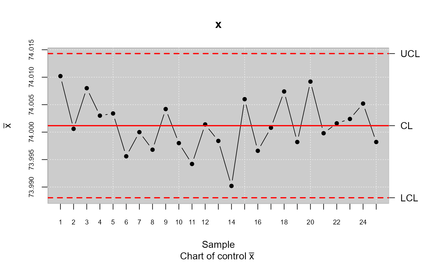
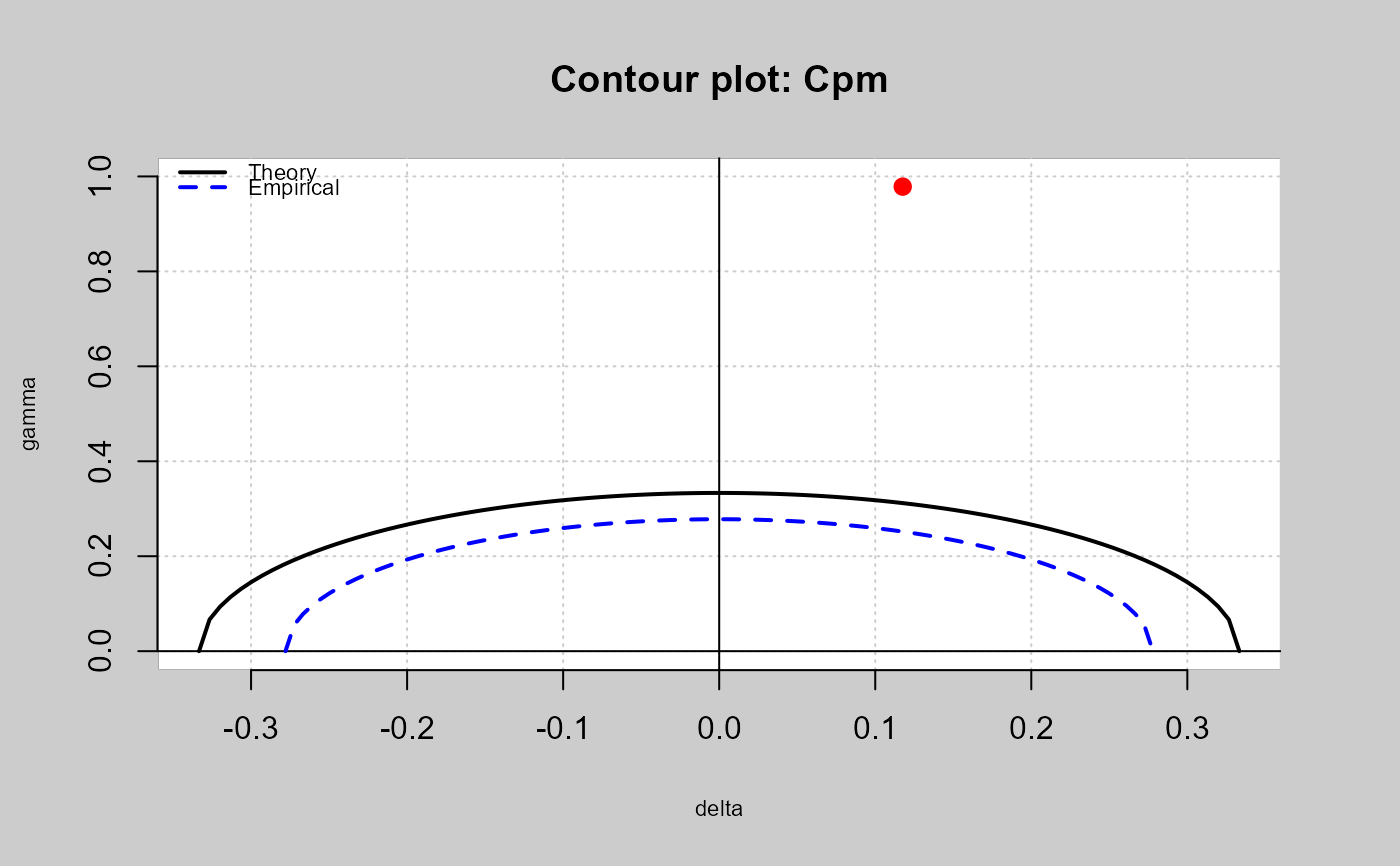
Process capability index (estimate Cpm)

Estimate "Cpm" using the method described by Kerstin Vannman(2001).

Usage

qcs.hat.cpm(
  object,
  limits = c(lsl = -3, usl = 3),
  target = NULL,
  mu = 0,
  std.dev = 1,
  nsigmas = 3,
  k0 = 1,
  alpha = 0.05,
  n = 50,
  contour = TRUE,
  ylim = NULL,
  ...
)

Arguments

object: qcs object of type "qcs.xbar" or "qcs.one".
limits: A vector specifying the lower and upper specification limits.
target: A value specifying the target of the process. If it is NULL, the target is set at the middle value between specification limits.
mu: A value specifying the mean of data.
std.dev: A value specifying the within-group standard deviation.
nsigmas: A numeric value specifying the number of sigmas to use.
k0: A numeric value. If the capacity index exceeds the k value, then the process is capable.
alpha: The significance level (by default alpha=0.05).
n: Size of the sample.
contour: Logical value indicating whether contour graph should be plotted.
ylim: The "y" limits of the plot.
...: Arguments to be passed to or from methods.

References

Montgomery, D.C. (1991) Introduction to Statistical Quality Control, 2nd ed, New York, John Wiley & Sons.
Vannman, K. (2001). A Graphical Method to Control Process Capability. Frontiers in Statistical Quality Control, No 6, Editors: H-J Lenz and P-TH Wilrich. Physica-Verlag, Heidelberg, 290-311.
Hubele and Vannman (2004). The E???ect of Pooled and Un-pooled Variance Estimators on Cpm When Using Subsamples. Journal Quality Technology, 36, 207-222.

Examples

library(qcr)
data(pistonrings) 
xbar <- qcs.xbar(pistonrings[1:125,],plot = TRUE)

mu <-xbar$center
std.dev <-xbar$std.dev
LSL=73.99; USL=74.01
qcs.hat.cpm(limits = c(LSL,USL),
           mu = mu,std.dev = std.dev,ylim=c(0,1))
qcs.hat.cpm(object = xbar, limits = c(LSL,USL),ylim=c(0,1))