This function is used to compute statistics required by the p chart.
Usage
qcs.p(x, ...)

# S3 method for default
qcs.p(
  x,
  var.index = 1,
  sample.index = 2,
  covar.index = NULL,
  covar.names = NULL,
  data.name = NULL,
  sizes = NULL,
  center = NULL,
  conf.nsigma = 3,
  limits = NULL,
  plot = FALSE,
  ...
)

# S3 method for qcd
qcs.p(x, center = NULL, conf.nsigma = 3, limits = NULL, plot = FALSE, ...)
Arguments
- x
An object of class "qcd".
- ...
Arguments passed to or from methods.
- var.index
A scalar with the column number corresponding to the observed data for the variable (the variable quality). Alternativelly can be a string with the name of the quality variable.
- sample.index
A scalar with the column number corresponding to the index fo each group (sample).
- covar.index
Optional. A scalar or numeric vector with the column number(s) corresponding to the covariate(s). Alternativelly it can be a character vector with the names of the covariates.
- covar.names
Optional. A string or vector of strings indicating the names for the covariate columns. Only valid if there is more than one column of data. By default, takes the names from the original object.
- data.name
A string specifying the name of the variable which appears on the plots. If not provided, it is taken from the object given as data.
- sizes
Optional. A value or a vector of values specifying the sample sizes associated with each group. For continuous data, the sample sizes are obtained counting the non-
NAelements of thesample.indexvector. For attribute variable the argument sizes is required.- center
A value specifying the center of group statistics or the ''target'' value of the process.
- conf.nsigma
A numeric value used to compute control limits, specifying the number of standard deviations (if
conf.nsigma> 1) or the confidence level (if 0 <conf.nsigma< 1).- limits
A two-values vector specifying control limits.
- plot
Logical value. If
TRUEa p chart should be plotted.
Examples
library(qcr)
data(orangejuice)
str(orangejuice)
#> 'data.frame':	54 obs. of  4 variables:
#>  $ D     : int  12 15 8 10 4 7 16 9 14 10 ...
#>  $ sample: int  1 2 3 4 5 6 7 8 9 10 ...
#>  $ size  : int  50 50 50 50 50 50 50 50 50 50 ...
#>  $ trial : logi  TRUE TRUE TRUE TRUE TRUE TRUE ...
attach(orangejuice)
#> The following objects are masked from orangejuice (pos = 3):
#>
#>     D, sample, size, trial
#> The following objects are masked from pistonrings (pos = 4):
#>
#>     sample, trial
#> The following objects are masked from pistonrings (pos = 5):
#>
#>     sample, trial
#> The following objects are masked from circuit:
#>
#>     sample, size, trial
#> The following objects are masked from orangejuice (pos = 7):
#>
#>     D, sample, size, trial

datos.qcd <- qcd(data = orangejuice, var.index = 1, sample.index = 2,
                sizes = size, type.data = "atributte")

res.qcs <- qcs.p(datos.qcd)
summary(res.qcs)
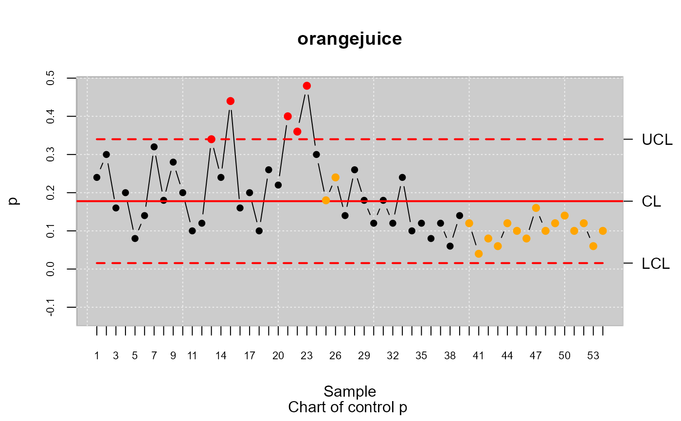
#> p chart for orangejuice
#>
#> Summary of group statistics:
#>        p
#>  Min.   :0.0400
#>  1st Qu.:0.1000
#>  Median :0.1400
#>  Mean   :0.1778
#>  3rd Qu.:0.2400
#>  Max.   :0.4800
#>
#> Group sample size:  50
#> Number of groups:  54
#> Center of group statistics:  0.1777778
#> Standard deviation:  0.3823256
#>
#> Control limits:
#>         LCL       UCL
#>  0.01557078 0.3399848
#>  0.01557078 0.3399848
#>  0.01557078 0.3399848
#>  0.01557078 0.3399848
#>  0.01557078 0.3399848
#>  0.01557078 0.3399848
#>  0.01557078 0.3399848
#>  0.01557078 0.3399848
#>  0.01557078 0.3399848
#>  0.01557078 0.3399848
#>  0.01557078 0.3399848
#>  0.01557078 0.3399848
#>  0.01557078 0.3399848
#>  0.01557078 0.3399848
#>  0.01557078 0.3399848
#>  0.01557078 0.3399848
#>  0.01557078 0.3399848
#>  0.01557078 0.3399848
#>  0.01557078 0.3399848
#>  0.01557078 0.3399848
#>  0.01557078 0.3399848
#>  0.01557078 0.3399848
#>  0.01557078 0.3399848
#>  0.01557078 0.3399848
#>  0.01557078 0.3399848
#>  0.01557078 0.3399848
#>  0.01557078 0.3399848
#>  0.01557078 0.3399848
#>  0.01557078 0.3399848
#>  0.01557078 0.3399848
#>  0.01557078 0.3399848
#>  0.01557078 0.3399848
#>  0.01557078 0.3399848
#>  0.01557078 0.3399848
#>  0.01557078 0.3399848
#>  0.01557078 0.3399848
#>  0.01557078 0.3399848
#>  0.01557078 0.3399848
#>  0.01557078 0.3399848
#>  0.01557078 0.3399848
#>  0.01557078 0.3399848
#>  0.01557078 0.3399848
#>  0.01557078 0.3399848
#>  0.01557078 0.3399848
#>  0.01557078 0.3399848
#>  0.01557078 0.3399848
#>  0.01557078 0.3399848
#>  0.01557078 0.3399848
#>  0.01557078 0.3399848
#>  0.01557078 0.3399848
#>  0.01557078 0.3399848
#>  0.01557078 0.3399848
#>  0.01557078 0.3399848
#>  0.01557078 0.3399848
#>
#> Beyond limits of control:
#> [1] 0.34 0.44 0.40 0.36 0.48
#>
#> Violationg runs:
#>  [1] 0.18 0.24 0.12 0.04 0.08 0.06 0.12 0.10 0.08 0.16 0.10 0.12 0.14 0.10 0.12
#> [16] 0.06 0.10
plot(res.qcs)


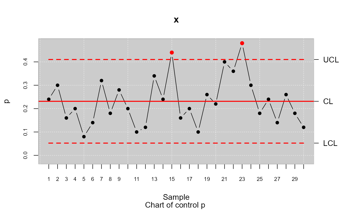
datos.qcs <- qcs.p(orangejuice[trial,c(1,2)], sizes = orangejuice[trial,3])
plot(datos.qcs)

