1. Examples of Interlaboratory Studies
An Interlaboratory Study evaluates the analytical methods performed by laboratories, either for the evaluation of the efficiency of the laboratories involved, or for the performance of an experimental procedure, or for the validation of a standard guideline. For example, to show the application of consistency test, the ILS, package contains the Glucose dataset, avalaible on ASTM E-691 that corresponds to the results of a clinical test. Likewise, from a study of the properties of the calcium oxolate material, three datasets (IDT, TG, DSC) were obtained, and they were incorporated into the package.
1.2. Clinical study of blood glucose measurement
The Glucose dataset corresponds to the serum glucose test (measurements of the concentration of glucose in the blood used to control the diabetes). In the study, eight laboratories where involved, and five different tests were performed on blood samples labelled with different references, ranging from a low sugar content to a very high one. Three replicates were obtained for each sample.
Each of these laboratories measured five different concentration levels (A, B, C, D, E) of a given material, and at each of these levels, three measurements were taken (3 replicates). Each laboratory provided a total of 15 measurements (3 for each level), therefore, with 8 laboratories involved, 120 measurements were obtained.
In order to access this dataset, the ILS package installing and loading is required. Once loading is performed, the Glucose data.frame object is called using the following instructions.
The first step to perform an analysis with the ILS package consist on using the function lab.qcdata() (quality control data) that receives a data.frame as an argument. The first column of the data frame must contain the response variable, the second column accounts for the index of repetition for each laboratory, the third column includes the index of the material at which the test was performed, while the fourth column includes the index of the laboratory where the procedure was performed.
Afterward, the qcdata object, corresponding to the lab.qcdata() class, is developed. The descriptive statistics information of the dataset can be summarized by using the summary() function.
qcdata <- lab.qcdata(Glucose)
summary(qcdata)
#>        x          replicate material   laboratory
#>  Min.   : 39.02   1:40      A:24     Lab1   :15
#>  1st Qu.: 78.45   2:40      B:24     Lab2   :15
#>  Median :135.03   3:40      C:24     Lab3   :15
#>  Mean   :149.09             D:24     Lab4   :15
#>  3rd Qu.:196.66             E:24     Lab5   :15
#>  Max.   :309.40                      Lab6   :15
#>                                      (Other):30
plot(qcdata, ylab = "Laboratory", xlab = "Glucose concentration in blood")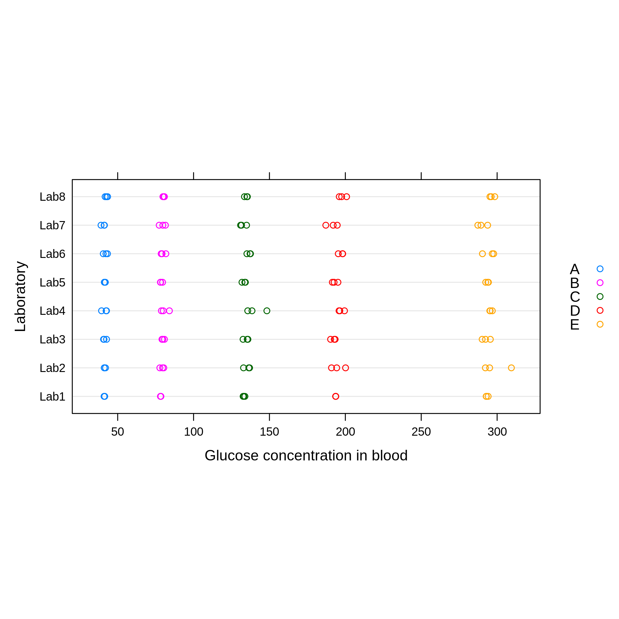
Figure 1, shows the results of all laboratories and it can be noted that the blood glucose level increases from material A to D and there is more variability between the results for each laboratory from the material C to material E.
In order to calculate the graphical and analytical statistics for the scalar (univariate) case, first, the function lab.qcs() (quality control statistics) has to be used. This function returns the estimation of the statistical required measures (mean, variance, etc.) for estimating the Mandel’s h and k statistics, as well as the required measures to perform the Cochran and Grubbs tests.
The qcdata object uses the lab.qcs() function to create the qcstat object that estimates both the mean and the global deviation from the results of all laboratories and all materials. In addition, the repeatability deviation (\(S_r\)) , the deviation between the means of laboratories (\(S_B\)), and the reproducibility deviation (\(S_R\)) for each material are estimated.
qcstat <- lab.qcs(qcdata)
summary(qcstat)
#>
#> Number of laboratories:  8
#> Number of materials:  5
#> Number of replicate:  3
#> Summary for Laboratory (means):
#>        Lab1      Lab2      Lab3      Lab4      Lab5      Lab6      Lab7
#> A  41.28333  41.44000  41.45000  41.45667  41.46333  42.02000  40.45667
#> B  78.31667  79.23333  79.90333  80.96333  78.69000  79.89333  79.51667
#> C 133.19667 135.40667 134.59000 140.83000 133.26667 136.61667 132.49333
#> D 193.65000 195.10667 192.09000 197.21333 193.05000 197.24333 191.26000
#> E 293.25333 298.91667 292.67000 295.82000 293.56333 294.95667 290.13667
#>        Lab8
#> A  42.57667
#> B  80.34667
#> C 134.71000
#> D 198.12333
#> E 296.62000
#>
#> Summary for Laboratory (Deviations):
#>        Lab1      Lab2      Lab3      Lab4      Lab5     Lab6     Lab7      Lab8
#> A 0.2230097 0.4850773 1.0608016 1.8117763 0.3666515 1.408119 1.247811 0.8224557
#> B 0.1582193 1.3268509 0.8303212 2.7660863 0.7754354 1.636592 2.059935 0.5064912
#> C 0.5909597 2.1679791 1.7287857 6.6200227 1.1987215 1.287025 2.124296 1.0343597
#> D 0.0600000 4.6824068 1.5932043 1.9365519 1.8826311 1.649616 3.817709 2.4637844
#> E 0.7266590 9.1869055 2.7101107 0.8835723 0.9543759 4.034282 3.304184 1.6479078
#>
#> Summary for Material:
#>        mean         S      S_r       S_B      S_R
#> A  41.51833 0.5543251 1.063224 0.6061274 1.058783
#> B  79.60792 0.8664835 1.496071 0.8627346 1.495481
#> C 135.13875 1.9071053 2.750879 2.6566872 3.478919
#> D 194.71708 1.4262962 2.625065 2.5950046 3.365713
#> E 294.49208 2.8067799 3.934974 2.6931364 4.192334
plot(qcstat, ylab = 'Material', xlab = 'Desviations')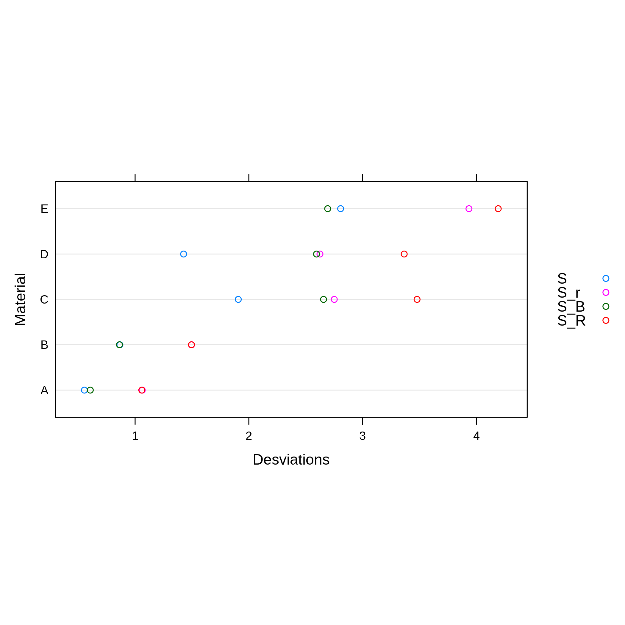
In Figure 2, the values of \(S\) (the global deviation of all laboratories), \(S_r\) (the repeatability’s deviation), \(S_R\) (reproducibility’s deviation) and \(S_B\) (the deviation between the means of the laboratories) are shown for each material. A greater variability can be noted from material C to material E. Materials C and D have a greater variability between the results of the laboratories (\(S_R\)) and within them (\(S_r\)).
1.2. Characterization of materials by thermogravimetric analysis
In a experiment, 105 samples of calcium oxalate were analysed by Thermogravimetric (TG) techniques, obtaining 105 TG curves showing the loss of oxalate mass as a function of temperature when the oxalate samples were heated at 20◦C/min. In addition, 90 samples of Calcium Oxalate were analysed by Differential Scanning Calorimetry (DSC) thermal technique, obtaining 90 DSC curves that determinate, from an SDT instrument, the difference of energy between a reference and the oxalate sample. We can observe the exchange of energy between the sample and the reference as a function of temperature when the latter vary as a linear function of the time defined by a slope of 20◦C/min. Two sets of data were generated from the results, a TG dataset, obtained from 7 different laboratories, and a DSC dataset, obtained from 6 different laboratories. In each laboratory 15 curves were analysed in 1000 observations.
In addition, from the TG curves, a third set of data called IDT (Initial Decomposition Temperature) was obtained, this is a parameter defined by the temperature at which the studied material losses the 5% of its weight when it is heated at a constant rate. This dataset is composed of the IDT values of calcium oxalate obtained from 7 different laboratories that analyses (each one) 15 oxalate samples. This dataset is an example of ILS study with scalar response, obtained by extracting just only one representative feature from the TG curve. It is important to stress that when a feature extraction process is performed, there is the risk of loosing relevant information and thus making erroneous findings.
Laboratories 1, 6, and 7 presented non-consistent results. In laboratory 1 a Simultaneous Thermal Analyzer (STA) was used with an out of phase calibration program. In laboratory 6 we used a simultaneous SDT analyser with an old calibration, and finally, in laboratory 7 we used a simultaneous SDT analyser with a bias into the temperature with respect to the real values (2◦C displaced with respect to the melting point of the zinc).
For the estimation of the functional statistics (for the performance of the graphical and analytical methods), the procedure was the same as for the scalar case. The ILS package provides the ils.fqcdata() (functional quality control data) function that developes an object that has the structure of a data.frame, in which each row represents a test result. The size of the data.frame is \(n \times l\), where \(n\) is the number of replicates performed by each laboratory, and \(l\) accounts for the number of laboratories that participate in the study. Specific functions were implemented to make plots and summaries of these type of objects.
Then, the function ils.fqcs() (functional quality control statistical) is needed for the estimation of some important statistical functional measures: functional mean, functional variance, etc. These are necessary for the estimation of the \(H(t)\) and \(K(t)\) and the \(d_H\) and \(d_K\) statistics.
To built an object of class ils.fqcdata, first we defined the grid in which the observations will be obtained. In this case, the 1000 points that compose the grid accounts for temperatures ranging from 40◦C to 850◦C. In Figure 3, the TG curves are presented. From the fqcdata object, the fqcstat object was performed.
delta <- seq(from = 40 ,to = 850 ,length.out = 1000 )
fqcdata <- ils.fqcdata(TG, p = 7, argvals = delta)
main <- "TG curves obtained from calcium oxalate"
xlab <- "Temperature (C)"
ylab <- "Mass (%)"
fqcstat <- ils.fqcs(fqcdata)
summary(fqcstat)
#>
#> Number of laboratories:  7
#> Number of replicates:  15
plot(x = fqcdata, main = main, xlab = xlab , ylab = ylab,
legend = TRUE,x.co = 20, y.co = 90)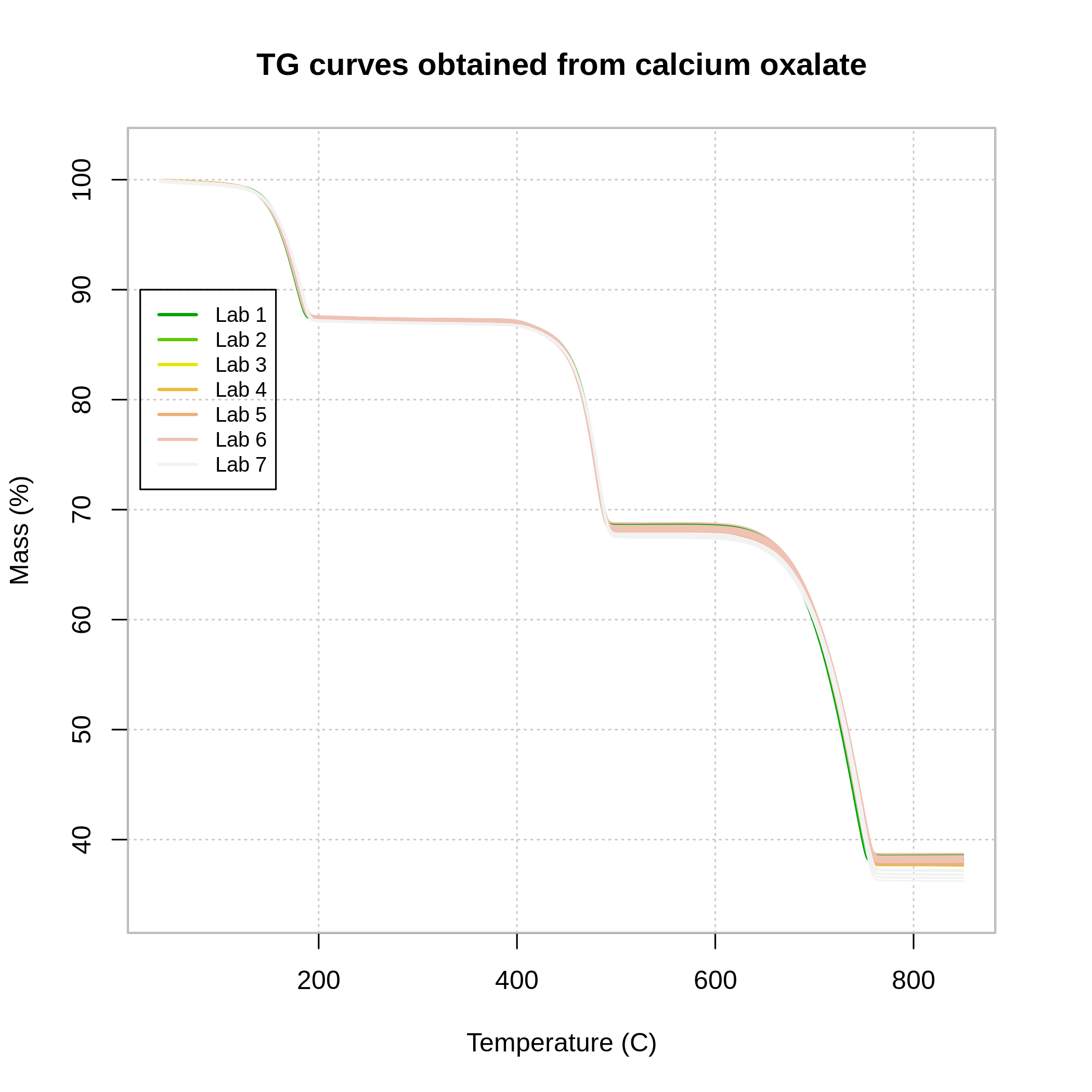
The plot() function creates a panel with four graphs, in the first row we have the means and functional variances for each laboratory, while in the second row the mean and global functional variance are plotted. Figure 4, shows the different functional means and functional variances for each laboratory, as well as the overall mean and the overall variance corresponding to the complete TG dataset.
plot(fqcstat, xlab = xlab, ylab = ylab)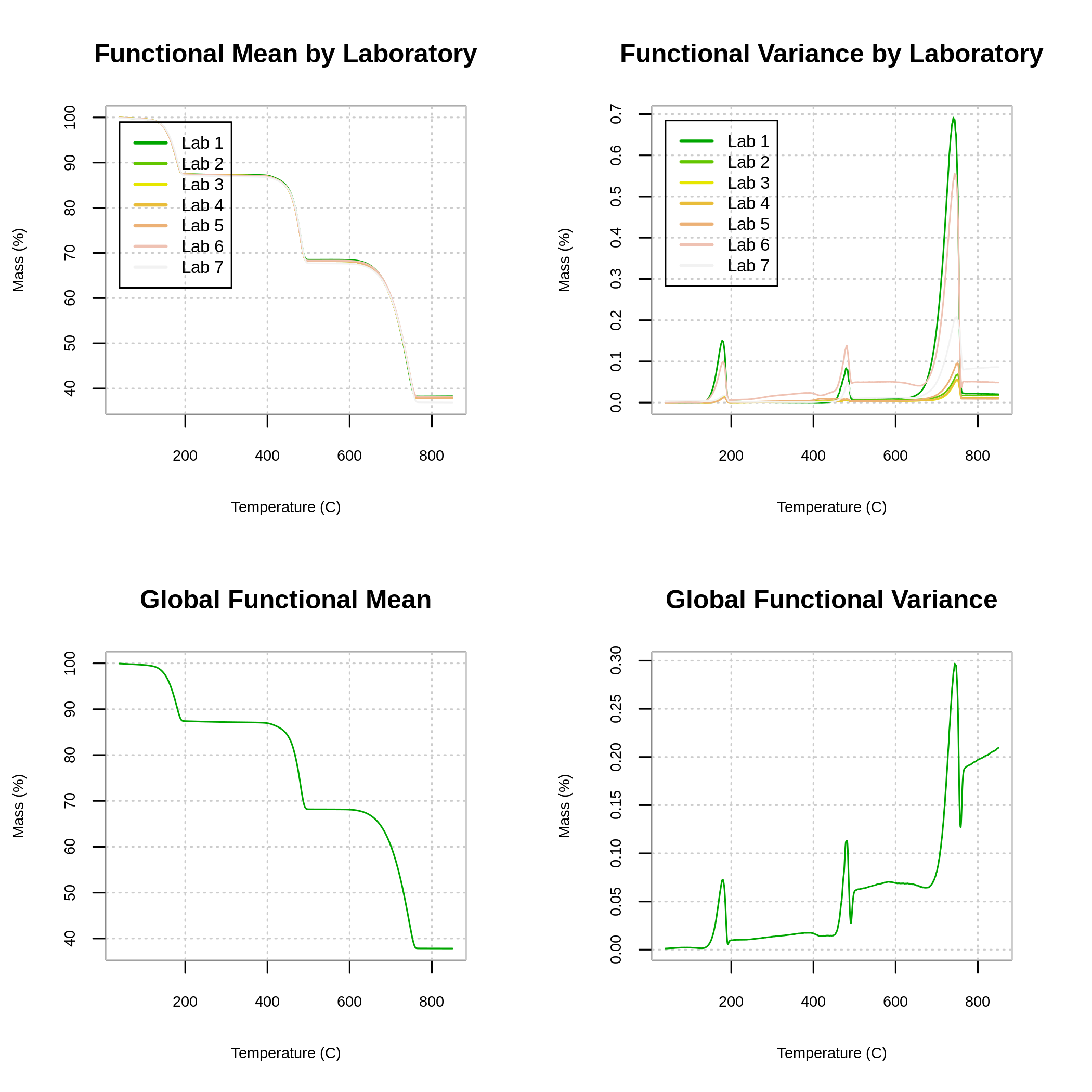
TG curves obtained from calcium oxalate.
Afterward, the qcdata object, corresponding to the lab.qcdata() class, is developed. The descriptive statistics information of the dataset can be summarized by using the summary() function. Figure 1, shows the results of all laboratories.